Importance of objective data assessment
Imagine throwing a six sided dice and writing down the numbers it lands on. If you got one ten times in a row, what would be the odds of getting it again? One in six, 100%, 0%, something else? And why? Would you question the dice? Maybe it’s faulty somehow, and gives only ones?
What if it landed on these numbers: 5463122365? Would you consider this result more fair, and not question the dice? You are probably aware that getting 1111111111 and 5463122365 have exactly the same probability. And that a chance of getting one as the eleventh result is the same as for the first, one in six. But somehow, 5463122365 seems more random. Apparently, there is a subjective feeling of randomness. Humans are not very good at assessing features of long streams of numbers. If we only had some kind of a machine which could do it faster, and with no bias.
Descriptive and inferential statistics
Descriptive statistics has been around for centuries, but it’s in overdrive lately, thanks to computers and big data. As the name suggests, its goal is to analyze and explain data. To attain any useful knowledge or attempt to predict future trends, which is a job of inferential statistics, we must first understand historical measurements. In general, business intelligence systems are tools which help us to describe and analyze the data we have. To be able to generalize some finding, we must have data which is representative of the whole group: if, for example, we are doing a survey on public perception of some product we are preparing for the market, we should include people of all ages. We need to make sure that although survey subject’s ages are random, we cover the whole range equally, as much as possible. This can be seen as the quality control of our data. Univariate analysis is focused on describing a single variable, like the age in our example.
Variable distribution
Uniform and normal distribution
Univariate distribution is defined as a function that provides probabilities of occurrence of possible outcomes of a variable. It is a summary of the frequency of the values. For discrete variables, this function describes the occurrence of individual values. In case of continuous variables, we split values in ranges.
Variable has the uniform distribution if any value has equal probability of occurrence. In our survey example, this would be the best type of distribution for subject ages: it would mean that we sampled all ages equally. This statement of “the best type of distribution” can be discussed. Not all ages are represented equally in the general population. We might not be interested in surveying infants, if we are aiming at selling the product. Maybe our product is not suitable for people with some types of disabilities, which are more common in certain age groups. It is crucial to understand the data, and what we expect from it.
Normal distribution is another very common type. Its graph forms a bell curve, which means that most frequent values are in the center, and the frequency gradually declines towards the ends of the possible values.
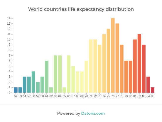
This peak in the graph is the most popular value, it represents the central tendency of our variable. Depending on our data, and what we are using it for, different variants of central tendency measure can be used.
Types of central tendencies
Mean, mode and median
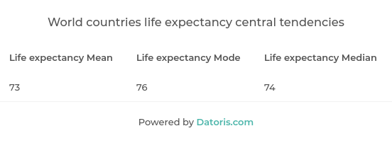
Mean is a simple average of our values. It is a sum of all the values, divided by their number. Mode represents a value which occurs most often. It can be undefined, if no value is repeated. Median is the middle value, we have to order our values and then pick the one in the middle.
Sometimes, comparing all three might give us some information as well. In our dice throwing example, if we had 1111661111 as a result of ten throws, mean would give us 2, mode would be 1, while median would give us 1, once the values are ordered. In this case, mean, although usually considered the most useful type of central tendency, shows us somewhat misleading value. We never got 2 on our dice, it might even not be possible, if the dice is faulty, but if we were asked which value is most common, we would have to answer it’s 2. In combination with mode and median however, it’s clear that our data is not evenly distributed. Median is usually least influenced by skewed data as it shows value in the middle, outliers get discarded. In normal distribution, all three measures are the same.
Dispersion
Range, variance, standard deviation
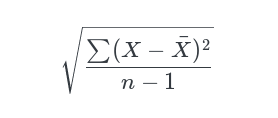
Variability, or dispersion, also has several variants, which can be used as complementary methods of describing and understanding the data. Range is the most common, and perhaps the simplest. It represents the difference between the largest and the lowest value. The variance is calculated by finding the difference between every value and the mean, squaring those differences, summing those up, and getting the average. Taking the square root from variance gives us standard deviation.
Summary statistics applications
Putting theory into practice
Descriptive statistics is simplifying the data in a way. Whenever we reduce our view of the data, we make our lives easier, because we don’t have to handle each value separately, but introduce new layers of approximation. Too many layers, or approximations done badly, and we are getting further away from the correct interpretation of the data. If done properly, descriptive statistics can expose many useful insights.
In business intelligence, our goal is decision making founded on knowledge we got from data. This decision making is our attempt of predicting the future. Knowledge it’s based on is collected by descriptive statistics. It can be interpreted numerically, or graphically.
In databases for example, it’s used to optimize reserved storage, organize data to improve performance and predict resources needed to execute queries. Weather forecasts, stock market strategies, machine learning algorithms, betting odds, all have to be based on good understanding of historical data.